Question

Derive the equation of motion with the graphical method.

Answer 1

Hint
We know that the three equations of motion form the backbone of classical mechanics, and have seen the derivation of the equations of motion using the calculus method. One drawback of the calculus method is that you need a different expression for deriving each equation of motion. This drawback is not present in the graphical method as only one velocity-time graph is enough for all the three equations of motion.
$m=\dfrac{\left( {{y}_{2}}-{{y}_{1}} \right)}{\left( {{x}_{2}}-{{x}_{1}} \right)}$ , $are{{a}_{trapezium}}=\dfrac{1}{2}\times (su{{m}_{parallel-sides}})\times (dis\tan c{{e}_{parallel-sides}})$

Complete step by step answer
The graph of velocity against time is drawn for an object that starts moving with an initial velocity $u$ and moves with certain acceleration $a$ and travels for time $t$ and has a final velocity $v$ when observed. The graph can be drawn as given

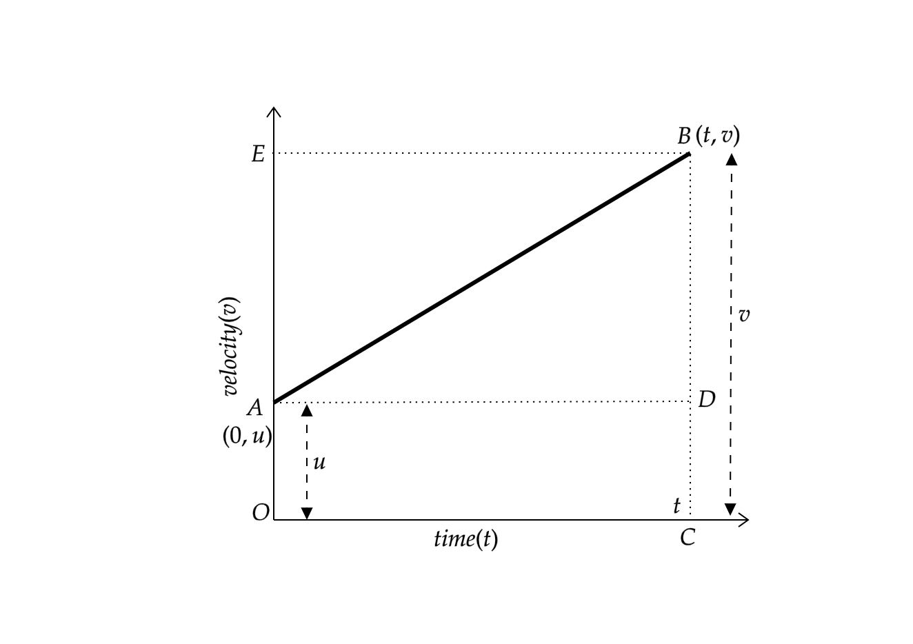
Now we all know that the slope of the curve of a velocity-time graph gives the acceleration of the particle and the area under the curve gives us the displacement of the particle.
The curve or the plot of the motion is given by the line AB; and since the co-ordinates of the points A and B are known, its slope can be given as
$m=\dfrac{\left( {{y}_{2}}-{{y}_{1}} \right)}{\left( {{x}_{2}}-{{x}_{1}} \right)}$
Now we know that this slope gives us the value of the acceleration of the particle, hence we can say
$\begin{align}
& a=\dfrac{\left( v-u \right)}{\left( t-0 \right)} \\
& \Rightarrow at=v-u \\
& \Rightarrow v=u+at \\
\end{align}$
This is the first equation of motion. Now the second equation of motion involves the displacement of the particle and we have discussed above that the area under the curve gives the displacement of the particle. Using this approach, we can say that the area of trapezium AOBC gives the displacement. We know that the area of a trapezium is given as half the product of the sum of the parallel sides and the distance between them.
For the given graph, we can say that
$displacement=\dfrac{1}{2}\times (OA+BC)\times (OC)$
Substituting the values of the mentioned sides, we get
$s=\dfrac{1}{2}\times (u+v)\times (t)--equation(a)$
Substituting the value of the final velocity from the first equation and simplifying, we get
$\begin{align}
& s=\dfrac{1}{2}\times (u+u+at)\times (t) \\
& \Rightarrow s=\dfrac{1}{2}\times \left( 2ut+a{{t}^{2}} \right) \\
& \Rightarrow s=ut+\dfrac{1}{2}a{{t}^{2}} \\
\end{align}$
This is the second equation of motion.
From the first equation of motion, we can say that $t=\dfrac{\left( v-u \right)}{a}$
Substituting this value of time in equation (a) obtained above, we get
$\begin{align}
& s=\dfrac{1}{2}\times (u+v)\times \dfrac{\left( v-u \right)}{a} \\
& \Rightarrow 2as=(v+u)(v-u) \\
& \Rightarrow 2as={{v}^{2}}-{{u}^{2}}\left[ \because (a+b)(a-b)={{a}^{2}}-{{b}^{2}} \right] \\
& \Rightarrow {{v}^{2}}={{u}^{2}}+2as \\
\end{align}$
This is the third equation of motion.
Thus we have successfully derived all the equations using the graphical method.

Note
We have three methods of deriving the equations of motion, namely the algebraic method, the graphical method and the calculus method. The algebraic method can be related very closely to the graphical method that we used in our solution above. The calculus method is used when the object changes its state over infinitesimal intervals of time and hence depicting the motion by a graph is not feasible.