Courses
Courses for Kids
Free study material
Offline Centres
More
Store Icon
Store

Statistics Class 11 Notes CBSE Maths Chapter 13 (Free PDF Download)

ffImage
banner

Revision Notes for CBSE Class 11 Maths Chapter 13 (Statistics) - Free PDF Download

Revising maths requires memorizing a lot of formulas and devising short-cuts to solve problems. You will get all of this along with prompt guidance from the teachers of Vedantu once you avail of our Notes of Class 11 Revision Notes Chapter 13. The subject matter experts of Vedantu solve these solutions with a step-by-step explanation that will help you clarify your concepts. These notes are also downloadable and printable, which makes them very handy.


Related Study Materials for Class 12 Maths Chapter 13


Chapter-wise Links for Mathematics Class 11 Notes


Related Important Links for Mathematics Class 11

Along with this, students can also download additional study materials provided by Vedantu for Maths Class 11–

Competitive Exams after 12th Science
tp-imag
bottom-arrow
tp-imag
bottom-arrow
tp-imag
bottom-arrow
tp-imag
bottom-arrow
tp-imag
bottom-arrow
tp-imag
bottom-arrow

Statistics Class 11 Notes Maths - Basic Subjective Questions


Section–A (1 Mark Questions)

1. What is the mean deviation of x observations x1,x2,x3,...,xn from their mean.

Ans. $M D=\frac{1}{n} \sum_{i=1}^n\left|x_i-\bar{x}\right|$.


2. If x1,x2,...,xn be n observations and $\bar{x}$ be their arithmetic mean. Then, what is the formula for the standard deviations.

Ans. The formula for $\mathrm{S} . \mathrm{D}=\sigma=\sqrt{\frac{\sum\left(x_i-\bar{x}\right)^2}{n}}$.


3. Coefficient of variation $=\frac{----}{Mean}\times 100$ .

Ans. $C V=\dfrac{S D}{\text { Mean }} \times 100$.


Hence, the value of the filler is SD.


4. If  $\bar{x}$ is the mean of n values of x, then $\sum_{i=1}^n\left(x_i-\bar{x}\right)$ is always equal to ..................

Ans. If $\bar{x}$ is the mean of $\mathrm{n}$ observations of $x$, then $\sum_{i=1}^n\left(x_i-\bar{x}\right)=0$ and if ' $a$ ' has the value other than $\bar{x}$, then $\sum_{i=1}^n\left(x_i-\bar{x}\right)^2$ is less then $\sum\left(x_i-a\right)^2$


5. If the variance of a data is 121, then the standard deviations of the data is ..................

Ans. We know that

$$S D=\sqrt{\text { variance }}=\sqrt{121}=11$$

Hence, the value of the filler is 11 .


Section–B (2 Marks Questions)

6. (i) The standard deviation of a data is ................... of any change in origin but is ..................... of change of scale.

(ii) The sum of squares of the deviations of the values of the variable is ................... when taken about their arithmetic mean.

Ans. (i) Since the standard deviation of any data is independent of any change in origin but is dependent of any change of scale. 

Hence, the value of the fillers are independent and dependent.

(ii) The sum of the squares of the deviations of the value of variable is minimum when taken about their arithmetic mean. Hence, the value of the filler is minimum.


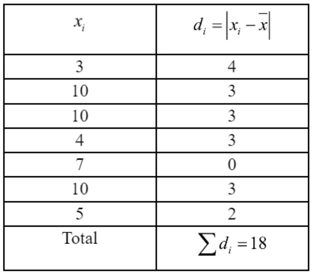
7. Find the mean deviation of the data 3, 10, 10, 4, 7, 10, 5 from the mean.

Ans.
Observations are given by $3,10,10,4,7$, 10 and 5

$$\begin{aligned}& \therefore \bar{x}=\frac{3+10+10+4+7+10+5}{7}=\frac{49}{7}=7 \\& M D=\frac{\sum d_i}{n}=\frac{18}{7}=2.57\end{aligned}$$


mean deviation of  data 3, 10, 10, 4, 7, 10, 5


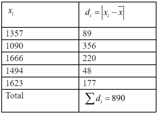
8. The lives (in hours) of 5 bulbs were noted as follows: 1357, 1090, 1666, 1494, 1623. Find the mean deviation (in hours) from their mean.

Ans. he lives of 5 bulbs are given by $1357,1090,1666,1494,1623$

$$\therefore \text { Mean }=\frac{1357+1090+1666+1494+1623}{5}$$

$$\Rightarrow \bar{x}=\frac{7230}{5}=1446$$

$$\therefore E=\frac{\sum d_i}{n}=\frac{890}{5}=178 \text {. }$$


Mean Deviation


9. If the mean of 100 observations is 50 and their standard deviation is 5, then find the sum of all the squares of all the observation.

Ans. Here $\bar{x}=\frac{\sum x_i}{n}$

$$\begin{aligned}& 50=\frac{\sum x_i}{100} \Rightarrow \sum x_i=5000 \\& \therefore S D=\sqrt{\frac{\sum x_i^2}{n}-\left(\frac{\sum x_i}{n}\right)^2} \\& 5=\sqrt{\frac{\sum x_i^2}{100}-\left(\frac{5000}{100}\right)^2} \Rightarrow25=\frac{\sum x_i^2}{100}-2500 \\& \Rightarrow \frac{\sum x_i^2}{100}=2500+25 \Rightarrow \frac{\sum x_i^2}{100}=2525 \\& \therefore \sum x_i^2=2525 \times 100=252500 .\end{aligned}$$


10. If x1,x2,x3,x4 and x5 be the observations with mean m and standard deviations S then, find the standard deviation of the observations Kx1, Kx2, Kx3, Kx4 and Kx5.

Ans. Here

$$\begin{aligned}& m=\frac{\sum x_i}{N}, S=\sqrt{\frac{\sum x_i^2}{5}-\left(\frac{\sum x_i}{5}\right)^2} \\& \therefore S D=\sqrt{\frac{K^2 \sum x_i^2}{5}-\left(\frac{K \sum x_i}{5}\right)^2} \\& =\sqrt{\frac{K^2 \sum x_i^2}{5}-K^2\left(\frac{\sum x_i}{5}\right)^2} \\& =K \sqrt{\frac{\sum x_i^2}{5}-\left(\frac{\sum x_i}{5}\right)^2} \\& =K \cdot S .\end{aligned}$$


11. Find the standard deviation for first 10 natural numbers as $f(x)=\frac{3x-4}{5}$  then write $f^{-1}(x)$ .

Ans.

$$11. We know that $\mathrm{SD}$ of first $\mathrm{n}$ natural numbers $\sqrt{\frac{n^2-1}{12}}$

Here $n=10$

$$\therefore S D=\sqrt{\frac{(10)^2-1}{12}}=\sqrt{\frac{99}{12}}=\sqrt{8.25}=2.87 \text {.}$$


12. The following information relates to a sample of total frequency 60: $\sum x^{2}=18000$  and $\sum x=960$ then find the variance.

Ans. We know that variance

$$\begin{aligned}& (\sigma)^2=\frac{\sum x_i^2}{N}-\left(\frac{\sum x_i}{N}\right)^2 \\& =\frac{18000}{60}-\left(\frac{960}{60}\right)^2=300-256=44 .\end{aligned}$$


13. The standard deviations of some temperature data in $^{\circ}C$  is 5. If the data were converted into $^{\circ}F$  then what would be the new variance.

Ans. Given that $\sigma_C=5$

We know that

$$\begin{aligned}& C=\frac{5}{9}(F-32) \Rightarrow F=\frac{9 C}{5}+32 \\& \therefore \sigma_F=\frac{9}{5} \sigma_C=\frac{9}{5} \times 5=9 \\& \therefore \sigma_F^2=(9)^2=81 .\end{aligned}$$


PDF Summary - Class 11 Maths Statistics (Chapter 13)Terminologies:


  • Statistics – It is the science of collection, organization, presentation, analysis and interpretation of the numerical data.

  • Limit of the class – The end values of a class is called its limits. The highest value is the upper limit and the lowest value is the lower limit.

  • Class interval – The difference between the upper and lower limit of each class.

  • Primary and secondary data – The data when collected by the investigator himself is termed as primary data and when it is collected by someone other than the investigator, then it is called the secondary data.

  • Variable or variate – A symbol or characteristic, whose magnitude varies from observation to observation is called a variable or variate. e.g., weight, height etc.

  • Frequency – The number of times a given observation occurs in a given set of data is called frequency of that observation.

  • Discrete frequency distribution – The frequency distribution in which the data is presented in a way that the exact measurements of the units are clearly visible is called a discrete frequency distribution.

  • Continuous frequency distribution – The frequency distribution in which the classes groups are not exactly measurable is called continuous frequency distribution.

  • Cumulative frequency distribution – The frequency obtained after adding the frequency of first class to the second class and then to the third class and so on, then the final frequency obtained is called the cumulative frequency. The frequencies given should be in the form of grouped or class frequencies.

Graphical Representation Of Frequency Distribution:

  • Histogram – A histogram is drawn by marking the given class intervals on x-axis and corresponding frequencies on y-axis. In the corresponding intervals, an erected rectangle is drawn having width proportional to the class interval and length proportional to the frequency of that class interval. When we take the class interval is taken as unit length on the graph, then the frequency of that class denotes the area of the rectangle.

When the class intervals are of unequal widths, then the height of the rectangles are proportional to the ratio of the frequencies to the width of each class. A sample of histogram has been shown below;


Histogram


  • Bar diagram – While drawing bar diagrams, only the length of bars or rectangles are taken into consideration. The data is divided into different classes, then the classes are marked with equal widths on the x-axis and then corresponding frequencies are marked on y-axis which in turn is proportional to the length of each bar. An example has been shown below;


Bar Diagram


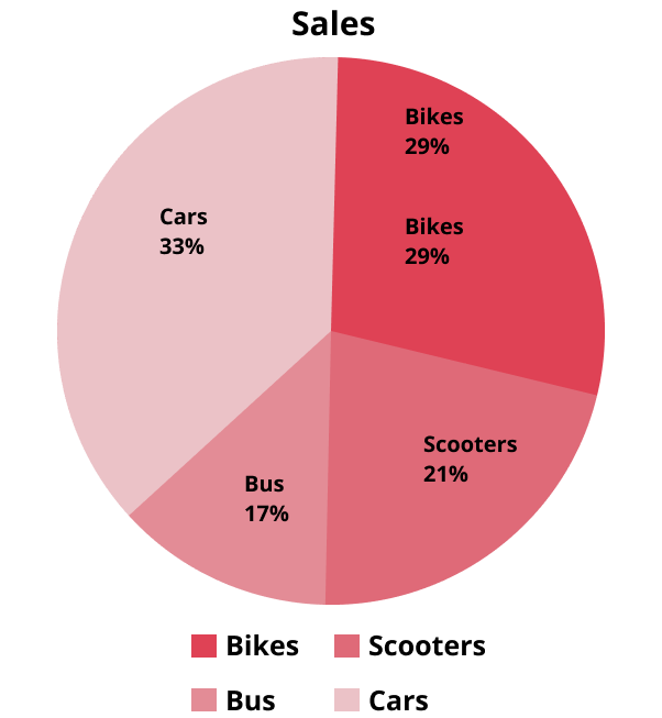
  • Pie diagrams – These are used to represent relative frequency distribution, in which a circle is divided into sectors which are equal to the number of classes and the area of each sector is proportional to the frequency of that class. The division is done by proportionately dividing the angles as per the frequencies. An example has been shown below;


Pie chart


To draw the required sectors, we find the central angles for that which can be calculated using the following relation;

$\text{Central angle}=\dfrac{Frequency\times {{360}^{{}^\circ }}}{\text{Total frequency}}$

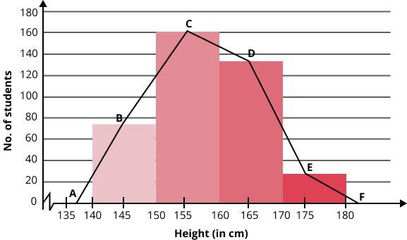
  • Frequency Polygon – In order to draw the frequency polygon of an ungrouped frequency distribution, the variate values are plotted on the x-axis and the corresponding frequencies are plotted on the y-axis. The mid-points of each bar are then joined using straight line to show a trend. An example has been shown below;


Frequency Polygon


  • Cumulative frequency curve (Ogive) – We first prepare a cumulative frequency table from the given data. Then we plot the cumulative frequencies against the lower or upper limits of the corresponding class intervals. Then, we join the points and the curve obtained is called a cumulative frequency curve or ogive. Ogives are generally drawn using two methods;

  • The ‘less than’ method – On the x-axis, plot the points with the upper limits and on the ordinates or y-axis, the corresponding less than cumulative frequencies. Then the points are joined by free hand to het a smooth curve or less than ogive. It is also called a falling curve.

  • The ‘more than’ method – On the x-axis, plot the points with the lower limits and on the ordinates or y-axis, the corresponding more than cumulative frequencies. Then the points are joined by free hand to het a smooth curve or less than ogive. It is also called a falling curve.

An example has been shown in the diagram below;


Cumulative Frequency Curve


Measures Of Central Tendency:

Measures of central tendency is the process of describing a complete data set by using a central value of that data set. The five measures of central tendency are enlisted below:

  • Arithmetic mean – It is the ratio of the sum of the vales of the items in a series to the total amount of data. These are further of five types;

i) Arithmetic mean for unclassified data – If we have $n$ numbers ${{x}_{1}},{{x}_{2}},{{x}_{3}},....,{{x}_{n}}$, then arithmetic mean is given by;

$A=\overline{X}=\dfrac{{{x}_{1}}+{{x}_{2}}+{{x}_{3}}+....+{{x}_{n}}}{n}$

$=\dfrac{\Sigma _{i=1}^{n}{{x}_{i}}}{n}$.

ii) Arithmetic mean for frequency distribution – If we have $n$ numbers ${{x}_{1}},{{x}_{2}},{{x}_{3}},....,{{x}_{n}}$, such that their corresponding frequencies are ${{f}_{1}},{{f}_{2}},{{f}_{3}},....,{{f}_{n}}$ respectively, then arithmetic mean is given by;

$A=\dfrac{{{f}_{1}}{{x}_{1}}+{{f}_{2}}{{x}_{2}}+{{f}_{3}}{{x}_{3}}+....+{{f}_{n}}{{x}_{n}}}{{{f}_{1}}+{{f}_{2}}+{{f}_{3}}+....+{{f}_{n}}}$

$=\dfrac{\Sigma _{i=1}^{n}{{x}_{i}}{{f}_{i}}}{\Sigma _{i=1}^{n}{{f}_{i}}}$.

iii) Arithmetic mean for classified data – Let us have a class interval with lower limit as $a$ and upper limit as $b$, then the class mark, $x=\dfrac{a+b}{2}$. Now, for a classified data, let the class marks be ${{x}_{1}},{{x}_{2}},{{x}_{3}},....,{{x}_{n}}$ be the variables of the classes, then the arithmetic mean is given by;

\[A=\dfrac{\Sigma xf}{\Sigma f}=\dfrac{\Sigma _{i=1}^{n}\dfrac{1}{2}\left( {{a}_{i}}+{{b}_{i}} \right)\times {{f}_{i}}}{\Sigma _{i=1}^{n}{{f}_{i}}}\].

Step deviation method;

\[A={{A}_{1}}+\left( \dfrac{\Sigma _{i=1}^{n}{{f}_{i}}{{u}_{i}}}{\Sigma _{i=1}^{n}{{f}_{i}}} \right)h\]

Where, ${{A}_{i}}$ is the assumed mean

${{u}_{i}}=\dfrac{{{x}_{i}}-{{A}_{1}}}{h}$

${{f}_{i}}=$frequency

$h=$width of interval

iv) Combined mean – If ${{x}_{1}},{{x}_{2}},{{x}_{3}},....,{{x}_{r}}$ be $r$ groups of observations, then we can find the arithmetic mean of the combined group $x$ using the formula,

$A=\dfrac{{{n}_{1}}{{A}_{1}}+{{n}_{2}}{{A}_{2}}+{{n}_{3}}{{A}_{3}}+....+{{n}_{r}}{{A}_{r}}}{{{n}_{1}}+{{n}_{2}}+{{n}_{3}}+....+{{n}_{r}}}$.

Where,

${{A}_{r}}=$Arithmetic mean of collection ${{x}_{r}}$

${{n}_{r}}=$total frequency of the collection ${{x}_{r}}$

v) Weighted arithmetic mean – The weighted arithmetic mean, if $w$ is the weight of the variable $x$ is given by;

${{A}_{w}}=\dfrac{\Sigma wx}{\Sigma w}$.

Properties Of Arithmetic Mean – 

a) Arithmetic means are always independent of change of origin and the change of scale.

b) The algebraic sum of deviations of a set of values with their arithmetic mean is zero.

c) When taken about mean, the sum of the squares of the deviations of a set of values is minimum.

  • Geometric Mean - If we have $n$ numbers ${{x}_{1}},{{x}_{2}},{{x}_{3}},....,{{x}_{n}}$, then geometric mean is given by;

$G={{\left( \prod\limits_{i=1}^{n}{{{x}_{i}}} \right)}^{\dfrac{1}{n}}}=\sqrt[n]{{{x}_{1}}.{{x}_{2}}.{{x}_{3}}......{{x}_{n}}}$ or

$G=anti\log \left[ \dfrac{\log {{x}_{1}}+\log {{x}_{2}}+...+\log {{x}_{n}}}{n} \right]$

For frequency distribution, we can have

$G={{\left( {{x}_{1}}{{f}_{1}}.{{x}_{2}}{{f}_{2}}.....{{x}_{n}}{{f}_{n}} \right)}^{\dfrac{1}{N}}}$

Where $N=\sum\limits_{i=1}^{n}{{{f}_{i}}}$

Or, $G=anti\log \left[ \dfrac{{{f}_{1}}\log {{x}_{1}}+{{f}_{2}}\log {{x}_{2}}+...+{{f}_{n}}\log {{x}_{n}}}{N} \right]$

  • Harmonic mean - If we have $n$ numbers ${{x}_{1}},{{x}_{2}},{{x}_{3}},....,{{x}_{n}}$, then harmonic mean is given by;

$HM=\dfrac{n}{\dfrac{1}{{{x}_{1}}}+\dfrac{1}{{{x}_{2}}}+...+\dfrac{1}{{{x}_{n}}}}=\dfrac{n}{\sum\limits_{i=1}^{n}{\dfrac{1}{{{x}_{i}}}}}$

If the corresponding frequencies are ${{f}_{1}},{{f}_{2}},{{f}_{3}},....,{{f}_{n}}$, then

$HM=\dfrac{{{f}_{1}}+{{f}_{2}}+{{f}_{3}}+....+{{f}_{n}}}{\dfrac{{{f}_{1}}}{{{x}_{1}}}+\dfrac{{{f}_{2}}}{{{x}_{2}}}+...+\dfrac{{{f}_{n}}}{{{x}_{n}}}}=\dfrac{\sum\limits_{i=1}^{n}{{{f}_{i}}}}{\sum\limits_{i=1}^{n}{\dfrac{{{f}_{i}}}{{{x}_{i}}}}}$

  • Median – When we arrange a given set of data in ascending or descending order, then the value lying in the middle is the median of the given data set. It is denoted by ${{M}_{d}}$ and is an average of the position of the numbers.

i) Median for simple distribution – In this type of distribution, first we arrange the terms in either in the ascending order or in the descending order and then find the number of terms $n$.

a) When $n$ is odd, then median is the $\left( \dfrac{n+1}{2} \right)th$ term.

b) When $n$ is even, there will be two terms in the middle. Then the median will be the mean of two middle terms $\dfrac{n}{2}th$ and $\left( \dfrac{n}{2}+1 \right)th$.

ii) Median for unclassified frequency distribution – First, find $\dfrac{N}{2}$, where $N=\Sigma {{f}_{i}}$. Then find the cumulative frequency of the data given and then see the value of the variable which is just greater than or equal to $\dfrac{N}{2}$. This value of the variable is called as the median.

iii) Median of classified data (median class) - First, find $\dfrac{N}{2}$. Then find the cumulative frequency of each class then see the value of the cumulative frequency that is just greater than or equal to $\dfrac{N}{2}$. The corresponding class is the median class.

For a continuous distribution, median is given by

${{M}_{d}}=l+\left( \dfrac{\dfrac{N}{2}-C}{f} \right)\times h$

Where, $l=$lower limit of the median class

$f=$frequency of the median class

$N=\sum{f}$=total frequency

$C=$cumulative frequency of the class preceding the median class

$h=$length of the median class

  • Quartiles – Like median, a distribution can also be divided into more equal parts (four, five, six etc.). The quartiles for a continuous distribution are given by

${{Q}_{1}}=l+\left( \dfrac{\dfrac{N}{4}-C}{f} \right)\times h$.

Where, $l=$lower limit of the quartile class

$f=$frequency of the quartile class

$N=$$\Sigma f$=total frequency

$C=$cumulative frequency of the class preceding the first quartile class

$h=$length of the quartile class

Similarly,

${{Q}_{3}}=l+\left( \dfrac{\dfrac{3N}{4}-C}{f} \right)\times h$.

  • Mode – The value at the point about which the data set tend to be most highly concentrated is called the mode ${{M}_{o}}$ of the distribution.

i) Mode for a raw data – Suppose we have the following numbers of a variable $70,80,90,96,70,96,96,90$, then the mode will be $96$ as it occurs maximum number of times. Graphically mode can be represented as follows;


Mode for Raw Data


ii) For classified distribution – In case of datasets divided into classes then the class with maximum frequency is called the modal class and the middle point of that modal class is called is called the crude mode. The class preceding and succeeding the modal class are called the pre-modal and post-modal class respectively.

iii) Mode for classified data (continuous distribution) – The mode is given by;

${{M}_{O}}=l+\left( \dfrac{{{f}_{0}}-{{f}_{1}}}{2{{f}_{0}}-{{f}_{1}}-{{f}_{2}}} \right)\times h$

Where, $l=$ lower limit of modal class

${{f}_{0}}=$ frequency of the modal class

${{f}_{1}}=$ frequency of the pre-modal class

${{f}_{2}}=$ frequency of the post-modal class

$h=$ length of class interval

  • Relation between mean, Median and Mode – 

i) $Mean-Mode=3\left( Mean-Median \right)$

ii) $Mode=3Median-2Mean$

Symmetrical And Skew Distribution:

A distribution is said to be symmetric if same number of frequencies is distributed on either side of the mode. In this case the frequency curve is bell-shaped and $A={{M}_{d}}={{M}_{o}}$.


Symmetric and Skew-Symmetric distribution


The variation does not have symmetry in the case of an anti-symmetric or skew distribution. Considering two cases,

(i) Positive skewness - The frequencies increases sharply in the beginning and decreases slowly after the modal value and $A > {{M}_{d}} > {{M}_{o}}$.


Positive Skewness


(ii) Negative skewness - The frequencies increases slowly in the beginning and decreases slowly after the modal value and $A < {{M}_{d}} < {{M}_{o}}$.


Negative skewness


Measure Of Dispersion:

Dispersion of the data is the degree to which numerical data tend to spread about an average value. There are three dispersions, enlisted below:

  • Range is used to denote the difference between the highest and the lowest element of a data. It can be represented as $range={{x}_{\max }}-{{x}_{\min }}$.

The coefficient of range is expressed as $\dfrac{{{x}_{\max }}-{{x}_{\min }}}{{{x}_{\max }}+{{x}_{\min }}}$.

It finds its uses in statists, especially in series relating to quality control in production.

i) Inter-quartile range is ${{Q}_{3}}-{{Q}_{1}}$.

ii) Semi-inter quartile range (quartile deviation) is QD = $\dfrac{{{Q}_{3}}-{{Q}_{1}}}{2}$ 

iii) Coefficient of quartile deviation is $\dfrac{{{Q}_{3}}-{{Q}_{1}}}{{{Q}_{3}}+{{Q}_{1}}}$

iv) \[QD=\dfrac{2}{3}SD\] 

  • Mean Deviation is defined as the arithmetic mean of absolute deviations of the values of the variable from a measure of their average, which can be either of mean, median, or mode. $\delta $ is used to denote it. The formula for various conditions is below,

i) For simple (discrete) distribution $\delta =\sum{\dfrac{\left| x-z \right|}{n}}$, where n is the number of terms and z can be either of A or ${{M}_{d}}$ or ${{M}_{o}}$.

ii) For unclassified frequency distribution $\delta =\dfrac{\sum \left| x-z \right|}{\sum f}$

iii) For classified distribution $\delta =\dfrac{\sum \left| x-z \right|}{\sum f}$, x is for class mark of the interval.

iv) $MD=\dfrac{4}{5}SD$

v) Average (mean or Median or Mode) $=\dfrac{mean\text{ }deviation\text{ }from\text{ }the\text{ }avergae}{average}$ 

vi) Coefficient of Mean Deviation is the ratio of MD and the mean from which the deviation is measured and is given by $MD=\dfrac{\sum \left| x-\overline{x} \right|}{n}$.

  • Standard deviation is defined as the square root of the arithmetic mean of the squares of deviations of the terms from their arithmetic mean. It is denoted by $\sigma $. The formulas are as below,

i) For simple distribution $\sigma =\sqrt{\dfrac{\sum {{\left( x-\overline{x} \right)}^{2}}}{n}}=\sqrt{\dfrac{\sum {{d}^{2}}}{n}}$.

ii) For frequency distribution $\sigma =\sqrt{\dfrac{\sum f{{\left( x-\overline{x} \right)}^{2}}}{\sum f}}=\sqrt{\dfrac{\sum f{{d}^{2}}}{\sum f}}$.

iii) For classified data $\sigma =\sqrt{\dfrac{\sum f{{\left( x-\overline{x} \right)}^{2}}}{\sum f}}=\sqrt{\dfrac{\sum f{{d}^{2}}}{\sum f}}$ x is the class mark.

iv) Shortcut Method for SD $\sigma =\sqrt{\dfrac{\sum f{{d}^{2}}}{\sum f}-{{\left( \dfrac{\sum fd}{\sum f} \right)}^{2}}}$, where \[d=x-A'\] and $A'$ is the assumed mean.

v) Standard deviation of the Combined Series – If ${{n}_{1}},{{n}_{2}}$ are the sizes, $\overline{{{X}_{1}}},\overline{{{X}_{2}}}$ are the means and ${{\sigma }_{1}},{{\sigma }_{2}}$ are the standard deviation of the series, then the standard deviation of the combined series is given by $\sigma =\sqrt{\dfrac{{{n}_{1}}\left( {{\sigma }_{1}}^{2}+{{d}_{1}}^{2} \right)+{{n}_{2}}\left( {{\sigma }_{2}}^{2}+{{d}_{2}}^{2} \right)}{{{n}_{1}}+{{n}_{2}}}}$ , where ${{d}_{1}}=\overline{{{X}_{1}}}-\overline{X}\text{ }and\text{ }{{d}_{2}}=\overline{{{X}_{2}}}-\overline{X}$ 

  • Variance is the square of standard deviation and ${{\sigma }^{2}}$ is used to denote it.

Analysis of Frequency Distributions:

  • The measure of variability is called as the coefficient of variation. It is independent of units. The letters C.V. is used for denoting it. It is defined as $C.V=\dfrac{\sigma }{\overline{x}}\times 100$, where the term $\dfrac{\sigma }{\overline{x}}$ is called coefficient of standard deviation.

  • The distribution for which the coefficient of variation is less is called more consistent.

  • For two series with equal means, the series with greater standard deviation is called more variable than the other. 

  • The series with lesser value of standard deviation is said to be more consistent than the other.

Notes of Statistics Class 11 Statistics – Brief Chapter Overview

Class 11 Maths Revision Notes Chapter 13 PDF

With the entire Class 11 Revision Notes Statistics available in PDF format on the official website of Vedantu, you have your mathematics revision at your fingertips. Download and save them on your device or print them out in a hard copy for a quick revision of all important formulas anytime, anywhere, even on the go without an internet connection. The Class 11 Statistics Notes are made keeping in mind the understanding level of class 11 students; hence you will be able to grasp all the problems discussed easily.

Revision Notes Class 11 Maths Chapter 13

Definition of Statistics and some Useful Terms - Statistics is used to collect, organize, and present numerical data for its analysis and interpretation. Some important terms associated with statistics are:

  • Limit of the Class - In a class, the smallest and the largest data values that can go in it are called the limit of the class.

  • Class Interval - It is also called the size of the class and is measured as the difference between the upper and lower limit of the class.

  • Primary and Secondary Data - The data which the investigator himself/herself collects is called the primary data. The data which others (not the investigator) collect is termed as secondary data.

  • Variable or Variate - Any parameter of the data whose magnitude changes from one observation to another is a variable. Examples of variates are age, weight, height, etc.

  • Frequency - The frequency of a given observation is the number of times it occurs in the data.

  • Discrete Frequency Distribution - If the exact measurements of units are clearly shown in the data presented, then that frequency distribution is termed as Discrete Frequency Distribution.

  • Continuous Frequency Distribution - If the exact measurements of units are not clear and data are presented as classes or groups, then that frequency distribution is termed as Continuous Frequency Distribution.

Graphical Representation of Frequency Distribution 

  • Histogram - To draw a histogram, all the class intervals are marked on the x-axis. Then vertical rectangles are erected on each interval. The height of these rectangles is proportional to the frequency distribution of that class group, and the area enclosed within each rectangle represents the frequency distribution of that class interval.

  • Bar Diagram - Bar diagrams are drawn by marking equal lengths on the x-axis for different classes. Only the bars' lengths are taken into consideration, which is proportional to the frequency distribution of that class.

  • Pie Diagrams - Pie diagrams are based on the relative frequency distribution. In a pie diagram, we draw a circle and then divide it into as numerous sectors as there are classes in a frequency distribution. The relative frequency of a class determines the area and angle of each sector.

  • Frequency Polygon - This is used to represent an ungrouped frequency distribution. Points are plotted whose abscissae is the variate value and ordinates are the frequencies. Then we join these points by a straight line to get the frequency polygon.

  • Arithmetic Mean - The arithmetic mean is calculated by summing the group of numbers and dividing it by the number of groups. It is denoted as:

  • For unclassified data, if there are n numbers as a1, a2, a3, …,an then it's AM = \[\overline{A}\] = (\[\sum_{i=1}^{n}\]ai)/n

  • If frequency distributions are known and f1, f2, f3, …, fn are the frequencies corresponding to a1, a2, a3, ...an then A = (\[\sum_{i=1}^{n}\]aifi)/\[\sum_{i=1}^{n}\]fi

  • For classified data, the class marks are taken as variables, and AM is defined as A = (\[\sum_{i=1}^{n}\]½ (xi + yi) * fi)/\[\sum_{i=1}^{n}\]fi. Here the class mark of the class interval is (x - y).

FAQs on Statistics Class 11 Notes CBSE Maths Chapter 13 (Free PDF Download)

1. What are the properties of arithmetic mean?

The properties of the arithmetic mean are:

  • The AM does not depend on the change of scale or origin.

  • If you algebraically sum the deviations of a set of values from their arithmetic mean, it is equal to 0.

  • If you sum the squares of deviations of a set of values, its value is the least when it is taken about their arithmetic mean.

2. What is the median of a distribution?

When the variables are arranged either in ascending or descending order, then the middle variable's value gives the median for that distribution. It is the average position of the numbers in the set. Formulas for simple distribution median are:

  • If there are odd numbers (n) then median Md = (n + 1)/2 th term.

  • If there are even numbers then there are two medians given by n/2th term and n/2 + 1th term.

3. What points should I consider while downloading the PDF file of revision notes of Chapter 13 of Class 11 Maths?

The method that should be obeyed for downloading the PDF file of Chapter 13 of Class 11 Maths is:

  • Tap on the given CBSE Class 11 Chapter 13 .

  • The link will open the official webpage of Vedantu.

  •  As the page appears, you will discover that the revision notes of Chapter 13 of Class 11 Maths are available on the website of Vedantu.

  •  At the peak of the webpage of Vedantu, you will see the “Download PDF” option.

  • Tap that option.

  • The PDF file of the notes will be downloaded.

4. What do you mean by the term statistics? Name some terminologies associated with statistics.

The organization, collection, presentation, interpretation and analysis of the numerical data are termed statistics.The different keywords associated with statistics are:

  • Class limit – These are of two types, upper and lower limits. The limit of a class is defined as the end value of a class.

  • The interval of Class – It is defined as the difference between the upper and lower limit of a class.

  • Primary data – It is the data collected by the researcher himself.

  • Secondary data – It is the data not collected by the investigator but collected by another person.

5. Describe the following terms:

  • Cumulative frequency distribution

  • Discrete frequency distribution

  • Continuous frequency distribution

  • Cumulative frequency distribution – The adding of the frequency of the first class, second class, third class and so on, which results in the final frequency is known as the cumulative frequency. For this frequency distribution, class frequencies are required.

  • Discrete frequency distribution – In this type of frequency distribution, the presentation of data is such that the measurements of the units are clearly visible.

  • Continuous frequency distribution – The type of frequency distribution in which groups of classes are not measurable is known as continuous frequency distribution.

If you want to understand these concepts more accurately then go through the given link CBSE Class 11 Chapter 13 .This link will redirect you to the official website of Vedantu where you can access the content related to Chapter 12 Straight lines for free. Additionally, you can also download its PDF if you want to study offline. 

6. What do you understand by the terms mean, median and mode?

(a) Mean – It is defined as the ratio of the sum of the values of items to the total quantity or amount of data. The types of arithmetic mean are:

  • Mean for unclassified data

  • Frequency distribution arithmetic mean

  •  Mean for combination

  • Mean for classified data

  • Arithmetic mean for weights

(b) Median – The middle value of the data set when the given data is arranged in ascending or descending order is known as the median.

(c) Mode – It is the value of that point at which the data set is highly concentrated.

7. Name some different types of graphical representations of frequency distribution.

  • Bar diagrams – In this graphical representation, the data is represented as rectangular bars. The length of these bars shows the value of different classes.

  • Histogram – It is the graphical representation in which the x-axis is assigned for class intervals and the y-axis is assigned for frequencies. Long rectangular bars are used to represent data.

  • Frequency polygon – This representation is used for ungrouped frequency distribution.

  • Pie diagrams – The representation in which a circle is divided into sectors to represent data or classes and frequency is known as a pie diagram.