Application of Derivatives Class 12 Notes: CBSE Maths Chapter 6

1. Derivative as Rate of Change

In various fields of applied mathematics, one has the quest to know the rate at which one variable is changing, with respect to another. The rate of change naturally refers to time. But we can have a rate of change with respect to other variables also. 

• An economist may want to study how the investment changes with respect to variations in interest rates.

• A physician may want to know how small changes in dosage can affect the body’s response to a drug.

• A physicist may want to know the rate of change of distance with respect to time.

All questions of the above type can be interpreted and represented using derivatives.

The average rate of change of a function:

The average rate of change of a function $f(x)$ with respect to $x$ over an interval $[a,a + h]$ is defined as $\dfrac{{f(a + h) - f(a)}}{h}$ .

Instantaneous rate of change of a function:

The instantaneous rate of change of a function$f$ with respect to $x$ is defined as

$f(x) = \mathop {\lim }\limits_{h \to 0} \dfrac{{f(a + h) - f(a)}}{h}$, provided the limit exists.

2. Equations Of Tangent & Normal

(I)The value of the derivative at $P\left( {{x_1},{y_1}} \right)$ gives the slope of the tangent to the curve at\[P\]Symbolically,

${f^\prime }\left( {{x_1}} \right) = {\left. {\dfrac{{dy}}{{dx}}} \right|_{({x_1},{y_1})}} = $ Slope of tangent at $P\left( {{x_1},{y_1}} \right) = m$ (say).

(II) Equation of tangent at $\left( {{x_1},{y_1}} \right)$ is $\left( {y - {y_1}} \right) = {\left( {\dfrac{{dy}}{{dx}}} \right)_{\left( {{x_1},{y_1}} \right)}} \times \left( {x - {x_1}} \right)$

(III) Equation of normal at $\left( {{x_1},{y_1}} \right)$ is $\left( {y - {y_1}} \right) = {\left( {\dfrac{{\dfrac{{ - 1}}{{dy}}}}{{dx}}} \right)_{\left( {{x_1},{y_1}} \right)}} \times \left( {x - {x_1}} \right)$

• The point $P\left( {{x_1},{y_1}} \right)$ will satisfy the equation of the curve and the equation of tangent and normal line.

• If the tangent at any point $P$ on the curve is parallel to $X$-axis then $\dfrac{{dy}}{{dx}} = 0$ at the point $P$.

• If the tangent at any point on the curve is parallel to $Y$-axis, then $\dfrac{{dy}}{{dx}} = \infty \,\,{\text{or}}\,\,\dfrac{{dx}}{{dy}} = 0$.

• If the tangent at any point on the curve is equally inclined to both the axes then $\dfrac{{dy}}{{dx}} =  \pm 1$.

• If the tangent at any point makes equal intercept on the coordinate axes then $\dfrac{{dy}}{{dx}} =  \pm 1$.

• Tangent to a curve at the point $P\left( {{x_1},{y_1}} \right)$ can be drawn even though $\dfrac{{dy}}{{dx}}$ at $P$ does not exist.

Example: $x = 0$ is a tangent to $y = {x^{\dfrac{2}{3}}}$ at $(0,0)$.

• If a curve passing through the origin is given by a rational integral algebraic equation, the equation of the tangent (or tangents) at the origin is obtained by equating to zero the terms of the lowest degree in the equation.

Example: If the equation of a curve be ${x^2} - {y^2} + {x^3} + 3{x^2}y - {y^3} = 0$, the tangents at the origin are given by ${x^2} - {y^2} = 0$ that is, $x + y = 0$ and $x - y = 0$.

(IV) (a) Length of the tangent $(PT) = \dfrac{{{y_1}\sqrt {1 + {{\left[ {{f^\prime }\left( {{x_1}} \right)} \right]}^2}} }}{{{f^\prime }\left( {{x_1}} \right)}}$

(b) Length of Subtangent $(MT) = \dfrac{{{y_1}}}{{{f^ {'}}\left( {{x_1}} \right)}}$

(c) Length of Normal $(PN) = {y_1}\sqrt {1 + {{\left[ {{f^\prime }\left( {{x_1}} \right)} \right]}^2}} $

(d) Length of Subnormal $(MN) = {y_1}{f^\prime }\left( {{x_1}} \right)$

(V) Differential:

The differential of a function is equal to its derivative multiplied by the differential of the independent variable. 

Thus if, $y = \tan x$ then $dy = {\sec ^2}xdx$

In general, $dy = {f^\prime }(x)dx$.

• $d(c) = 0$ where ' ${\text{c}}$ ' is a constant.

• $d(u + v - w) = du + dv - dw$

• $d(uv) = udv + vdu$

• The relation $dy = {f^\prime }(x)dx$ can be written as $\dfrac{{dy}}{{dx}} = {f^\prime }({\text{x}})$; thus the quotient of the differentials of $y$ and $x$ is equal to the derivative of $y$ with respect to $x$.

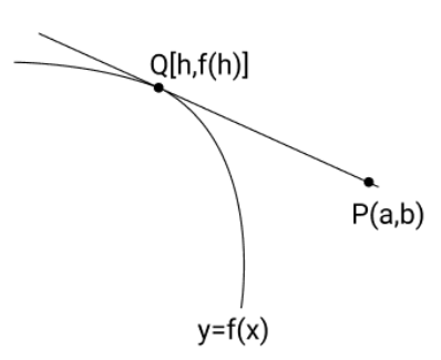
3. Tangent From an External Point

Given a point $P(a,b)$ which does not lie on the curve $y = f(x)$, then the equation of possible tangents to the curve $y = f(x)$, passing through $(a,b)$ can be found by solving for the point of contact $Q$.

And equation of tangent is $y - b = \dfrac{{f(\;h) - b}}{{h - a}}(x - a)$

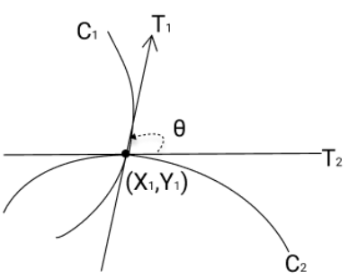
4. Angle Between The Curves

The angle between two intersecting curves is defined as the acute angle between their tangents or the normals at the point of intersection of two curves.

$\tan \theta  = \left| {\dfrac{{{m_1} - {m_2}}}{{1 + {m_1}\;{m_2}}}} \right|$

Here, ${m_1}\,\,{\text{and}}\,\,{{\text{m}}_2}$ are the slopes of tangents at the intersection point $\left( {{x_1},{y_1}} \right)$.

• The angle is defined between two curves if the curves are intersecting. This can be ensured by finding their point of intersection or by graphically.

• If the curves intersect at more than one point then the angle between curves is found out with respect to the point of intersection.

• Two curves are said to be orthogonal if the angle between them at each point of intersection is the shortest right angle, that is, ${m_1}\;{m_2} =  - 1$.

5. Shortest Distance Between Two Curves

Shortest distance between two non-intersecting differentiable curves is always along their common normal.

6. Errors and Approximations

(a) Errors

Let $y = f(x)$

From definition of derivative, $\mathop {\lim }\limits_{ax \to 0} \dfrac{{\delta y}}{{\delta x}} = \dfrac{{dy}}{{dx}}$ 

$\dfrac{{\delta y}}{{\delta x}} = \dfrac{{dy}}{{dx}}$ approximately

or $\delta {\text{y}} = \left( {\dfrac{{{\text{dy}}}}{{{\text{dx}}}}} \right).\delta {\text{x}}$ approximately 

Definition:

(i) $\delta x$ is known as absolute error in $x$.

(ii) $\dfrac{{\delta x}}{x}$ is known as relative error in $x$.

(iii) $\dfrac{{\delta x}}{x} \times 100$ is known as the percentage error in $x$.

• $\delta {\text{x}}$ and $\delta {\text{y}}$ are known as differentials.

7.Definitions

1.A function $f(x)$ is called an Increasing Function at a point $x$ $ = {\text{a}}$ if in a sufficiently small neighborhood around $x = a$. We have

\[f(a + h) > f(a)\]

\[f(a - h) < f(a)\]

Similarly Decreasing Function if

$f(a + h) < f(a)$

$f(a - h) > f(a)$

Above statements hold true irrespective of whether $f$ is non derivable or even 

discontinuous at $x = a.$

2. A differentiable function is called increasing in an interval $(a,b)$ if it is increasing at every point within the interval (but not necessarily at the endpoints). A function decreasing in an interval $(a,b)$ is similarly defined.

3. A function which in a given interval is increasing or decreasing is called "Monotonic" in that interval.

4. Tests for increasing and decreasing of a function at a point :

If the derivative ${f^\prime }(x)$ is positive at a point $x = a$, then the function $f(x)$ at this point is increasing. If it is negative, then the function is decreasing.

• Even if ${f^\prime }(a)$ is not defined, $f$ can still be increasing or decreasing.

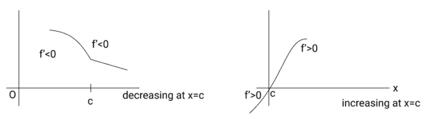
• ${f^\prime }({\text{c}})$ is not defined in both cases.

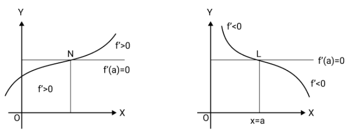
If ${f^\prime }(a) = 0$, then for $x = a$ the function may be still increasing or it may be decreasing as shown. It has to be identified by a separate rule.

Example:$f(x) = {x^3}$ is increasing at every point. Note that, $\dfrac{{dy}}{{dx}} = 3{x^2}$

• If a function is invertible it has to be either increasing or decreasing.

• If a function is continuous, the intervals in which it rises and falls may be separated by points at which its derivative fails to exist.

• If \[f\] is increasing in $[a,b]$ and is continuous then $f(b)$ is the greatest and $f(a)$ is the least value of $f$ in \[\left[ {a,{\text{ }}b} \right].\] Similarly if $f$ is decreasing in \[[a,b]\] then $f(a)$ is the greatest value and $f(b)$ is the least value.

5. (A) Rolle's Theorem:

Let $f(x)$ be a function of $x$ subject to the following conditions:

(i) $f({\text{x}})$ is a continuous function of ${\text{x}}$ in the closed interval of $a \leqslant x \leqslant b$

(ii) ${f^\prime }({\text{x}})$ exists for every point in the open interval $a < x < b$

(iii) $f({\text{a}}) = f(\;{\text{b}})$

Then there exists at least one point $x = c$ such that $a < c < b$ where ${f^\prime }(c) = 0$

(b) LMVT Theorem:

Let $f(x)$ be a function of $x$ subject to the following conditions:

(i) $f(x)$ is a continuous function of $x$ in the closed interval of $a \leqslant x \leqslant b$.

(ii) ${f^\prime }({\text{x}})$ exists for every point in the open interval $a < x < b$

Then there exists at least one point $x = c$ such that $a < c < b$ where ${f^\prime }(c) = \dfrac{{f(\;b) - f(a)}}{{b - a}}$

Geometrically, the slope of the secant line joining the curve at $x = a\,\,{\text{and}}\,\,x = b$ is equal to the slope of the tangent line drawn to the curve at $x = c$.

Note the following : Rolle's theorem is a special case of LMVT since

$f(a) = f(b) \Rightarrow {f^\prime }(c) = \dfrac{{f(b) - f(a)}}{{b - a}} = 0$.

• Physical Interpretation of LMVT: Now $[f(b) - f(a)]$ is the change in the function $f$ as $x$ changes from \[a\] to $b$ so that $\dfrac{{f(b) - f(a)}}{{b - a}}$ is the average rate of change of the function over the interval \[\left[ {a,{\text{ }}b} \right].\] Also ${f^\prime }(c)$ is the actual rate of change of the function for $x = c$. Thus, the theorem states that the average rate of change of a function over an interval is also the actual rate of change of the function at some point of the interval. In particular, for instance, the average velocity of a particle over an interval of time is equal to the velocity at some instant belonging to the interval.

This interpretation of the theorem justifies the name "Mean Value" for the theorem.

(c) Application of rolles theorem for isolating the real roots of an equation $f(x) = 0$

Suppose $a\,\& \,\;b$ are two real numbers such that ;

(i) $f(x){\text{ }}\& $ its first derivative ${f^\prime }(x)$ are continuous for $a \leqslant x \leqslant b$

(ii) $f(a)$ and $f(b)$have opposite signs

(iii) \[{f^\prime }(x)\]is different from zero for all values of $x$ between $a\,\& \,b$.

Then there is one and only one real root of the equation $f(x) = 0$ between $a\,\& \,b$.

8.How Maxima & Minima are Classified

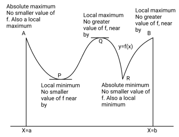
1.A function $f(x)$ is said to have a local maximum at $x = a$ if $f(a)$ is greater than every other value assumed by $f(x)$ in the immediate neighbourhood of $x = a$. 

Symbolically

$\left. {\begin{array}{*{20}{l}} {f(\;a) > f(\;a + h)} \\ {f(\;a) > f(\;a - h)}  \end{array}} \right] $ \Rightarrow x = a$ gives maxima for a sufficiently small positive $h$.

Similarly, a function $f(x)$ is said to have a local minimum value at $x = b$ if $f(\;{\text{b}})$ is least than every other value assumed by $f(x)$ in the immediate neighborhood at $x = b$. Symbolically if

$\left. {\begin{array}{*{20}{l}} {f(\;b) < f(\;b + h)} \\ {f(\;b) < f(\;b - h)}  \end{array}} \right] \Rightarrow x = b$ gives minima for a sufficiently small positive $h$.

(image will be uploaded)

• The local maximum and local minimum values of a function are also known as local/relative maxima or local/relative minima as these are the greatest and least values of the function relative to some neighborhood of the point in question.

• The term 'extremum' is used both for maxima or minima.

• A local maximum (local minimum) value of a function may not be the greatest (least) value in a finite interval.

• A function can have several local maximum and local minimum values and a local minimum value may even be greater than a local maximum value.

• Maxima and minima of a continuous function occur alternately and between two consecutive maxima, there is a minima and vice versa.

2. A necessary condition for maxima and minima

If $f(x)$ is a maxima or minima at $x = c$ and if ${f^\prime }(c)$ exists then ${f^\prime }(c) = 0$.

• The set of values of $x$ for which ${f^\prime }(x) = 0$ are often called stationary points. The rate of change of function is zero at a stationary point.

• In case ${f^\prime }(c)$ does not exist, $f(c)$ may be a maxima or minima and in this case, left-hand and right-hand derivatives are of opposite signs.

• The greatest (global maxima) and the least (global minima) values of a function $f$ in an interval \[[a,b]\] are $f(a)$ or $f(b)$ or are given by the values of $x$ which are critical points.

• Critical points are those where :

      (i) $\dfrac{{dy}}{{dx}} = 0$, if it exists; 

      (ii) or it fails to exist

3.Sufficient condition for extreme values First Derivative Test

$\left. {\begin{array}{*{20}{l}} {{f^\prime }(c - h) > 0} \\  {{f^\prime }(c + h) < 0}  \end{array}} \right] \Rightarrow x = c$ is a point of local maxima

Where $h$ is a sufficiently small positive quantity.

Similarly,

$\left. {\begin{array}{*{20}{l}} {{f^\prime }(c - h) < 0} \\  {{f^\prime }(c + h) > 0}  \end{array}} \right] \Rightarrow x = c$ is a point of local minima,

Where $h$ is a sufficiently small positive quantity.

Note : $ - {f^\prime }(c)$ in both the cases may or may not exist. If it exists, then ${f^\prime }(c) = 0$.

• If ${f^\prime }(x)$ does not change sign that is, it has the same sign in a certain complete neighbourhood of \[c\], then $f(x)$ is either strictly increasing or decreasing throughout this neighbourhood implying that $f(c)$ is not an extreme value of $f$.

4.Use of second order derivative in ascertaining the maxima or minima

(a) $f(c)$ is a minima of the function $f$, if ${f^\prime }(c) = 0\,\,\& \,\,{f^{\prime \prime }}(c) > 0$

(b) $f(c)$ is a maxima of the function $f$, if ${f^\prime }(c) = 0\,\,\& \,\,{f^{\prime \prime }}(c) < 0$

• If ${f^{\prime \prime }}(c) = 0$ then the test fails. Revert back to the first-order derivative check for ascertaining the maxima or minima.

5. Summary-working rule

• First: When possible, draw a figure to illustrate the problem & label those parts that are important in the problem. Constants and variables should be clearly distinguished. 

• Second: Write an equation for the quantity that is to be maximized or minimized. If this quantity is denoted by $'y'$, it must be expressed in terms of a single independent variable $x$. This may require some algebraic manipulations.

• Third : If $y = f(x)$ is a quantity to be maximum or minimum, find those values of $x$ for which $\dfrac{{dy}}{{dx}} = {f^\prime }(x) = 0$

• Fourth: Test each value of $x$ for which ${f^\prime }(x) = 0$ to determine whether it provides a maxima or minima or neither.

The usual tests are :

(a) If $\dfrac{{{d^2}y}}{{d{x^2}}}$ is positive when $\dfrac{{dy}}{{dx}} = 0$

$ \Rightarrow y$ is minima.

If $\dfrac{{{d^2}y}}{{d{x^2}}}$ is negative when $\dfrac{{dy}}{{dx}} = 0$

$ \Rightarrow y$ is maxima.

If $\dfrac{{{d^2}y}}{{d{x^2}}} = 0$ when $\dfrac{{dy}}{{dx}} = 0$, the test fails.

(b) If $\left. {\begin{array}{*{20}{l}} {{\text{ }}\,\,\,\,\,\,\,\,\,\,\,\,\,\,\,\,{\text{positive }}}&{{\text{ for }}x < {x_0}} \\  {\dfrac{{dy}}{{dx}}{\text{ is}}\,\,\,\,\,{\text{ zero }}}&{{\text{ for }}x = {x_0}} \\  {{\text{ }}\,\,\,\,\,\,\,\,\,\,\,\,\,\,\,\,{\text{negative }}}&{{\text{ for }}x > {x_0}}  \end{array}} \right] \Rightarrow $ a maxima occurs at $x = {x_0}$.

But if $\dfrac{{dy}}{{dx}}$ changes sign from negative to zero to positive as $x$ advances through ${x_0}$, there is a minimum. If $\dfrac{{dy}}{{dx}}$does not change sign, neither a maxima nor a minima. Such points are called INFLECTION POINTS.

• Fifth : If the function $y = f(x)$ is defined for only a limited range of values $a \leqslant x \leqslant b$ then examine $x = a\,\,\& x = b$ for possible extreme values.

• Sixth: If the derivative fails to exist at some point, examine this point as possible maxima or minima.

(In general, check at all Critical Points).

• If the sum of two positive numbers $x$ and $y$ is constant than their product is maximum if they are equal, i.e. $x + y = c,x > 0,y > 0$, then $xy = \dfrac{1}{4}\left[ {{{(x + y)}^2} - {{(x - y)}^2}} \right]$

• If the product of two positive numbers is constant then their sum is least if they are equal.

${(x + y)^2} = {(x - y)^2} + 4xy$

6.Significance of the sign of 2nd order derivative and points of inflection

The sign of the ${2^{{\text{nd }}}}$ order derivative determines the concavity of the curve. Such points such as $C\,\,\& \,\,E$ on the graph where the concavity of the curve changes are called the points of inflection. From the graph we find that if:

(image will be uploaded)

(i) $\dfrac{{{d^2}}}{{d{x^2}}} > 0 \Rightarrow $ Concave upwards

(ii) $\dfrac{{{d^2}}}{{d{x^2}}} < 0 \Rightarrow $ Concave downwards.

At the point of inflection we find that $\dfrac{{{d^2}}}{{d{x^2}}} = 0$ and $\dfrac{{{d^2}}}{{d{x^2}}}$ changes sign.

Inflection points can also occur if $\dfrac{{{d^2}}}{{d{x^2}}}$ fails to exist (but changes its sign). 

For example, consider the graph of the function defined as,

$f(x) = \left[ {\begin{array}{*{20}{c}} {{x^{3/5}}}&{{\text{  for }}x \in ( - \infty ,1)} \\  {2 - {x^2}}&{{\text{for }}x \in (1,\infty )} \end{array}} \right.$

• The graph below exhibits two critical points one is a point of local maximum 

$(x = c)$ and the other a point of inflection $(x = 0)$. This implies that not every Critical Point is a point of extrema.

Important Formulas of Class 12 Chapter 6 Application of Derivatives You Shouldn’t Miss!

1.Derivative of a Function:

\[\frac{d}{dx}[f(x)] = f'(x)\]

2. Critical Points:

To find the critical points of $ f(x) $, solve $ f'(x) = 0 $.

3. First Derivative Test:

For a function $ f(x) $:

If $ f'(x) $ changes from positive to negative at $ x = c $, then $ f(c) $ is a local maximum.

If $ f'(x) $ changes from negative to positive at $ x = c $, then $ f(c) $ is a local minimum.

4. Second Derivative Test:

For $ f(x) $:

If $ f''(x) > 0 $ at $ x = c $, then $ f(c) $ is a local minimum.

If $ f''(x) < 0 $ at $ x = c $, then $ f(c) $ is a local maximum.

If $ f''(x) = 0 $, the test is inconclusive.

5. Concavity:

$ f(x) $ is concave up if $ f''(x) > 0 $.

$ f(x) $ is concave down if $ f''(x) < 0 $.

6. Point of Inflection:

A point where $ f''(x) = 0 $ and $ f''(x) $ changes sign.

7. Derivative of Implicit Functions:

If $ F(x, y) = 0 $, then

\[\frac{dy}{dx} = -\frac{F_x}{F_y}\]

8. Maxima and Minima of Functions:

• For finding absolute maxima and minima on an interval [a, b]:

• Evaluate f(x) at critical points in (a, b) and endpoints a and b.

9. Optimization Problems:

• To solve optimization problems, set up the function to be maximized or minimized, find the derivative, and solve f'(x) = 0.

Importance of Application of Derivatives Class 12 Notes

The importance of Application of Derivatives Class 12 notes lies in their role as a key resource for understanding how derivatives are used to solve real-world problems and analyse mathematical functions. Here’s why these notes are crucial:

1. Simplified Learning: Application of derivatives can be a complex topic, but well-structured notes break down the concepts into manageable sections, making it easier for students to grasp and remember.

2. Exam Preparation: The notes focus on important formulas, key concepts, and problem-solving techniques that are frequently tested in board exams. This ensures students are well-prepared to tackle a variety of exam questions.

3. Foundation for Higher Studies: Understanding the application of derivatives is essential for higher studies in fields like engineering, economics, and physics. These notes lay the groundwork for advanced topics that students will encounter in college and competitive exams.

4. Practical Problem-Solving: The notes provide step-by-step explanations and examples of how derivatives are applied to find maxima and minima, solve rate-of-change problems, and determine tangents and normals. This practical approach helps students develop strong analytical and problem-solving skills.

5. Quick Revision Tool: The notes are concise and organized, making them an excellent tool for quick revision before exams. They highlight the most important points, allowing students to efficiently review the material.

Tips for Learning the Class 12 Maths Chapter 6 Application of Derivatives

Here are some useful tips for learning Class 12 Maths Chapter 6, "Application of Derivatives":

1. Review Basic Differentiation Concepts: Before diving into the applications, make sure you have a solid understanding of basic differentiation techniques. This includes mastering derivative rules such as the power rule, product rule, quotient rule, and chain rule.

2. Understand the Geometrical Interpretation: Derivatives can be used to find the slope of a tangent to a curve at a given point. Grasp the geometrical meaning of the derivative, which is crucial for solving problems related to the slope of curves and tangents.

3. Focus on Real-Life Applications: Study the real-life applications of derivatives, such as calculating rates of change, finding maximum and minimum values of functions, and solving problems related to motion, growth, and decay.

4. Master the Concepts of Maxima and Minima: Spend extra time understanding how to find local maxima and minima of functions using the first and second derivative tests. Practice problems where you need to identify and interpret these critical points.

5. Work on Increasing and Decreasing Functions: Learn how to determine intervals on which a function is increasing or decreasing by using the first derivative. This is a key concept that is often tested in exams.

6. Practice Problems on Tangents and Normals: Derivatives are used to find the equations of tangents and normals to a curve at a given point. Practice these types of problems extensively, as they frequently appear in exams.

7. Understand Rate of Change: Derivatives represent the rate of change of a quantity. Practice problems that involve finding the rate of change of one variable with respect to another, such as velocity, acceleration, and growth rates.

8. Use Graphical Analysis: Whenever possible, try to visualize the problem using graphs. This can help you better understand the behavior of functions and the application of derivatives in analyzing those behaviors.

Conclusion

Mastering the topic of Application of Derivatives is essential for success in Class 12 Mathematics and beyond. The comprehensive notes on Application of Derivatives provide clear explanations, key formulas, and step-by-step problem-solving techniques that simplify this complex subject. By using these notes for study and revision, students can build a strong understanding of the Application of Derivatives, enhance their problem-solving skills, and approach exams with confidence. These notes not only prepare students for board exams but also lay a solid foundation for higher studies in mathematics, engineering, and related fields.

Related Study Materials for Class 12 Maths Chapter 6 Application of Derivatives

Students can also download additional study materials provided by Vedantu for Class 12 Maths Chapter 6 Application of Derivatives:

Chapter-wise Revision Notes Links for Class 12 Maths

Important Study Materials for Class 12 Maths