


How to Apply Taylor’s Theorem to Solve Real Math Problems
In this article, Taylor's Theorem and its proof are discussed in detail. Taylor’s Theorem is used to express the value of a function as a sum of infinite terms that are calculated from the values of the derivatives of the function at a single point. Quantitative estimates of error are given by Taylor’s Theorem.
In this article, we will discuss the theorem along with proof, statement, and solved examples. We will also cover its limitations and applications in real life and in books. Some frequently asked questions by the readers are also answered at the end of the article.
Table of Contents
Introduction to Taylor's Theorem
History of Brook Taylor
Statement of Taylor's Theorem
Proof of Taylor's Theorem
Limitation of Taylor's Theorem
Applications of Taylor's Theorem
History of Brook Taylor

Brook Taylor
Image credit: Wikimedia
Name: Brook Taylor
Born: 18 August 1685
Died: 29 December 1731
Field: Mathematics
Nationality: British
Statement of Taylor's Theorem
Consider a function either real or composite, $f(x)$ that is differentiable.
Then, the power series for that function is described using the Taylor series as:
$f(x)=f(a) \dfrac{f^{\prime}(a)}{1 !}(x-a)+\dfrac{f^{\prime \prime}(a)}{2 !}(x-a)^{2}+\dfrac{f^{(3)}(a)}{3 !}(x-a)^{3}+\ldots$
which can be written as:
$f(x)=\sum_{n=0}^{\infty} \dfrac{f^{n}(a)}{n !}(x-a)^{n}$
where, $f^{(n)}(a)$ represents $n^{\text {th }}$ derivative of $f$
and $n$! represents the factorial of $n$.
Proof of Taylor's Theorem
We know the power series for any function is defined as follows:
$f(x)=\sum_{n=0}^{\infty} a_{n} x^{n}=a_{0}+a_{1} x+a_{2} x^{2}+a_{3} x^{3}+\ldots$
At $x=0$,
$f(x)=a_{0}$
Differentiating the given function:
$f^{\prime}(x)=a_{1}+2 a_{2} x+3 a_{3} x^{2}+4 a_{4} x^{3}+\ldots$
Substitute $x=0$ in the above equation, and we get:
$f^{\prime}(0)=a_{1}$
Differentiating again, we get
$f^{\prime \prime}(x)=2 a_{2}+6 a_{3} x+12 a_{4} x^{2}+\ldots$
Substituting $x=0$ in second-order differentiation
$f^{\prime \prime}(0)=2 a_{2}$
Therefore, $\dfrac{f^{\prime \prime}(0)}{2 !}=a_{2}$
Generalising the equation,
we have: $\dfrac{f^{n}(0)}{n !}=a_{n}$
Substitute the values in the power series:
$f(x)=f(0)+f^{\prime}(0) x+\dfrac{f^{\prime \prime}(0)}{2 !} x^{2}+\dfrac{f^{\prime} n(0)}{3 !} x^{3}+\ldots$
Generalising $f$ in the general form again, we get:
$f(x)=b+b_{1}(x-a)+b_{2}(x-a)^{2}+b_{3}(x-a)^{3}+\ldots$
At $x=a$, we have
$b_{n}=\dfrac{f^{n}(0)}{n !}$
Now, substituting the value of $b_{n}$ in a generalised form,
$f(x)=f(a) \dfrac{f^{\prime}(a)}{1 !}(x-a)+\dfrac{f^{\prime \prime}(a)}{2 !}(x-a)^{2}+\dfrac{f^{(3)}(a)}{3 !}(x-a)^{3}+\ldots$
Hence, Taylor's Theorem Formula is proved.
Taylor's Theorem for Two Variables
If $f(x, y)$ has continuous partial derivatives up to the nth order in a neighbourhood of a point $(a, b)$, then
$f(a+h, b+k)=f(a, b)+\left[h \dfrac{\partial}{\partial x}+k \dfrac{\partial}{\partial y}\right] f(a, b)+\dfrac{1}{2 !}\left[h \dfrac{\partial}{\partial x}+k \dfrac{\partial}{\partial y}\right]^{2} f(a, b)$
$+\dfrac{1}{3 !}\left[h \dfrac{\partial}{\partial x}+k \dfrac{\partial}{\partial y}\right]^{3} f(a, b)+\ldots \ldots+\dfrac{1}{(n-1) !}\left[h \dfrac{\partial}{\partial x}+k \dfrac{\partial}{\partial y}\right]^{n-1} f(a, b)+R_{n}$
Where,
$R_{n}=\dfrac{1}{n !}\left[h \dfrac{\partial}{\partial x}+k \dfrac{\partial}{\partial y}\right]^{n} f(a+\theta h, b+\theta k)$ for some $\theta: 0<\theta<1$
Here $R_{n}$ is called the remainder after $n$ times.
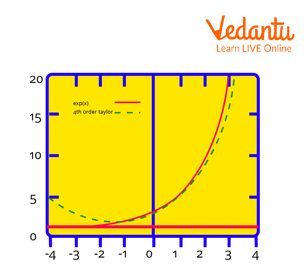
The Exponential Function y = ex
Limitation of Taylor's Theorem
Taylor's theorem is not applicable in the case of non-differentiable functions.
Applications of Taylor's Theorem
Taylor's Theorem is used in electric power systems to analyse power flow.
Taylor’s Theorem is also a multivariate theorem used in optimisation techniques in operation research.
Taylor’s Theorem approximates the value of the function at any point with the help of values of the function at one point only and, hence, reduces a lot of mathematical computational work.
Solved Examples
1. Find the first 4 terms of the Taylor series for the $\ln x$ function centred at $a=1$
Ans.
$f(x)=\ln x$ So,
$\Rightarrow f^{(1)}(x)=\dfrac{1}{x}$
$\Rightarrow f^{(2)}(x)=-\dfrac{1}{x^{2}}$
$\Rightarrow f^{(3)}(x)=\dfrac{2}{x^{3}}$
$\Rightarrow f^{(4)}(x)=-\dfrac{6}{x^{4}}$
and so on $\ln x=\ln 1+(x-1) \times 1+\dfrac{(x-1)^{2}}{2 !} \times(-1)+\dfrac{(x-1)^{3}}{3 !} \times(-2)+\ldots$
$\Rightarrow(x-1)-\dfrac{(x-1)^{2}}{2}+\dfrac{(x-1)^{3}}{3}-\dfrac{(x-1)^{4}}{4}+\ldots$
2.Find the first 4 terms of the Taylor series for the $\dfrac{1}{x}$ function centered at $a=1$
Ans.
$\Rightarrow f(x)=\dfrac{1}{x}$
So
$\Rightarrow f^{(1)}(x)=-\dfrac{1}{x^{2}}$
$\Rightarrow f^{(2)}(x)=\dfrac{2}{x^{3}}$
$\Rightarrow f^{(3)}(x)=-\dfrac{6}{x^{4}}$
and so
$\Rightarrow \dfrac{1}{x}=1+(x-1) \times(-1)+\dfrac{(x-1)^{2}}{2 !} \times(2)+\dfrac{(x-1)^{3}}{3 !} \times(-6)+\cdots$
$\Rightarrow 1-(x-1)+(x-1)^{2}-(x-1)^{3}-\cdots$
3. Find the first 4 terms of the Taylor series for the $\sin x$ function centred at $x=\dfrac{\pi}{4}$
Ans.
$f(x)=\sin x$.
So,
$\Rightarrow f'(x)=\cos x\\\Rightarrow f''(x)= -sinx\\\Rightarrow f'''(x)= - cosx\\$
and so
$\Rightarrow \sin x=\dfrac{\sqrt{2}}{2}+\left(x-\dfrac{\pi}{4}\right) \times\left(\dfrac{\sqrt{2}}{2}\right)+\dfrac{\left(x-\dfrac{\pi}{4}\right)^{2}}{2 !} \times\left(-\dfrac{\sqrt{2}}{2}\right)+\dfrac{\left(x-\dfrac{\pi}{4}\right)^{3}}{3 !} \times\left(-\dfrac{\sqrt{2}}{2}\right)+\cdots $
$\Rightarrow \dfrac{\sqrt{2}}{2}\left(1+\left(x-\dfrac{\pi}{4}\right)-\dfrac{\left(x-\dfrac{\pi}{4}\right)^{2}}{2}-\dfrac{\left(x-\dfrac{\pi}{4}\right)^{3}}{6}+\cdots\right)$
Conclusion
In the article, we have learned to State and Prove Taylor's Theorem PDF, the detailed proof of Taylor's Series Theorem, and solved questions related to the theorem. The expression for Taylor’s Series and Taylor's Theorem for Two Variables is discussed in detail. And the applications of the theorem shows us that the theorem has a wide range of application and importance in our day-to-day life besides Mathematics.
Important Formula to Remember
Taylor’s Series of a function around a point a is defined as:
$f(x)=\sum_{n=0}^{\infty} \dfrac{f^{n}(a)}{n !}(x-a)^{n}$
where $f$ is a function of $x$ and $a$ is any fixed point.
Related Links
FAQs on Taylor’s Theorem Explained with Proofs, Examples & Uses
1. What do you mean by Maclaurin’s Theorem\Series?
Maclaurin’s Series is a special case of Taylor’s Theorem. Taylor’s Theorem approximates the value of the function at all values, and Maclaurin's Series approximates the value of the function at zero only. In other words, we can say that if Taylor’s Series is centred at zero that the series is Maclaurin’s Series. On substituting $a=0$ in Talor's Series, we get Maclaurin's Series:
$f(x)=f(0) \dfrac{f^{\prime}(0)}{1 !}(x)+\dfrac{f^{\prime \prime}(0)}{2 !}(x)^{2}+\dfrac{f^{(3)}(0)}{3 !}(x)^{3}+\ldots$
2. Can we write Taylor’s Series for non-differentiable functions?
No, Taylor’s Series is based on the application of derivatives only. We can write Taylor’s Series for only differentiable functions. If any function is not differentiable, then we can not find the value of the derivatives of the function at a given point and hence, will not be able to write the Taylor’s Series for that function. If the function is a single variable or multivariable function, differentiability is the essential condition for Taylor’s series for both real and complex functions.
3. What is the difference between Taylor’s Series and Taylor’s Polynomial?
There is a minute difference between Taylor’s Series and Taylor’s Polynomial. Taylor’s Series is a series expressed as the sum of an infinite number of terms not necessarily carrying any value, i.e., the terms can also be zero.
On the other hand, Taylor’s Polynomial is a polynomial that is expressed as the sum of a finite number of terms. However, zero can also be a polynomial which is often referred to as Zero Polynomial. Taylor’s Polynomial can be written using the finite terms from Taylor’s Series.