


How do you graph \[y = \cot x\]?
Answer
556.8k+ views
Hint: We need to graph the given function. We will use the domain and some values of \[x\] lying between \[ - 2\pi \] and \[2\pi \] to find some values of \[y\]. Then, we will observe the behavior of the value of \[y\], and use it and the coordinates obtained to graph the function.
Complete step-by-step solution:
The domain of the function \[y = \cot x\] is given by \[\left\{ {x:x \in R{\rm{ and }}x \ne n\pi ,n \in Z} \right\}\]. This means that the cotangent of any multiple of \[\pi \] does not exist.
The graph of the cotangent function reaches arbitrarily large positive or negative values at these multiples of \[\pi \].
Now, we will find some values of \[y\] for some values of \[x\] lying between \[ - 2\pi \] and \[2\pi \].
Substituting \[x = - \dfrac{{3\pi }}{2}\] in the function \[y = \cot x\], we get
\[\begin{array}{l}y = \cot \left( { - \dfrac{{3\pi }}{2}} \right)\\ \Rightarrow y = 0\end{array}\]
Substituting \[x = - \dfrac{\pi }{2}\] in the function \[y = \cot x\], we get
\[\begin{array}{l}y = \cot \left( { - \dfrac{\pi }{2}} \right)\\ \Rightarrow y = 0\end{array}\]
Substituting \[x = \dfrac{\pi }{2}\] in the function \[y = \cot x\], we get
\[\begin{array}{l}y = \cot \left( {\dfrac{\pi }{2}} \right)\\ \Rightarrow y = 0\end{array}\]
Substituting \[x = \dfrac{{3\pi }}{2}\] in the function \[y = \cot x\], we get
\[\begin{array}{l}y = \cot \left( {\dfrac{{3\pi }}{2}} \right)\\ \Rightarrow y = 0\end{array}\]
The value of \[y\] at \[x = 2\pi ,\pi ,0,\pi ,2\pi \] is infinite.
Arranging the values of \[x\] and \[y\] in a table and writing the coordinates, we get
The value of \[y = \cot x\] decreases from \[\infty \] to 0 at \[x = - \dfrac{{3\pi }}{2}\], and then to \[ - \infty \] in the interval \[\left( { - 2\pi , - \pi } \right)\].
Similarly, the value of \[y = \cot x\] decreases from \[\infty \] to 0 at \[x = - \dfrac{\pi }{2},\dfrac{\pi }{2},\dfrac{{3\pi }}{2}\], and then to \[ - \infty \] in the intervals \[\left( { - \pi ,0} \right)\], \[\left( {0,\pi } \right)\], and \[\left( {\pi ,2\pi } \right)\].
Now, we will use the points \[\left( { - \dfrac{{3\pi }}{2},0} \right)\], \[\left( { - \dfrac{\pi }{2},0} \right)\], \[\left( {\dfrac{\pi }{2},0} \right)\], \[\left( {\dfrac{{3\pi }}{2},0} \right)\] and the behaviour of the value of \[y = \cot x\] to graph the function.
Therefore, we get the graph
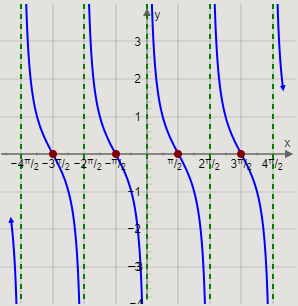
This is the required graph of the function \[y = \cot x\].
Note:
The period of the function \[y = \cot x\] is \[\pi \]. This means that the graph of \[y = \cot x\] will repeat for every \[\pi \] distance on the \[x\]-axis. It can be observed that the pattern and shape of the graph of \[y = \cot x\] is the same from \[ - 2\pi \] to \[ - \pi \], from \[ - \pi \] to 0, from 0 to \[\pi \], and from \[\pi \] to \[2\pi \]. The range of cotangent functions is from \[ - \infty \] to \[\infty \]. As tangent function is a reciprocal function cotangent function, so their graph faces opposite to each other.
Complete step-by-step solution:
The domain of the function \[y = \cot x\] is given by \[\left\{ {x:x \in R{\rm{ and }}x \ne n\pi ,n \in Z} \right\}\]. This means that the cotangent of any multiple of \[\pi \] does not exist.
The graph of the cotangent function reaches arbitrarily large positive or negative values at these multiples of \[\pi \].
Now, we will find some values of \[y\] for some values of \[x\] lying between \[ - 2\pi \] and \[2\pi \].
Substituting \[x = - \dfrac{{3\pi }}{2}\] in the function \[y = \cot x\], we get
\[\begin{array}{l}y = \cot \left( { - \dfrac{{3\pi }}{2}} \right)\\ \Rightarrow y = 0\end{array}\]
Substituting \[x = - \dfrac{\pi }{2}\] in the function \[y = \cot x\], we get
\[\begin{array}{l}y = \cot \left( { - \dfrac{\pi }{2}} \right)\\ \Rightarrow y = 0\end{array}\]
Substituting \[x = \dfrac{\pi }{2}\] in the function \[y = \cot x\], we get
\[\begin{array}{l}y = \cot \left( {\dfrac{\pi }{2}} \right)\\ \Rightarrow y = 0\end{array}\]
Substituting \[x = \dfrac{{3\pi }}{2}\] in the function \[y = \cot x\], we get
\[\begin{array}{l}y = \cot \left( {\dfrac{{3\pi }}{2}} \right)\\ \Rightarrow y = 0\end{array}\]
The value of \[y\] at \[x = 2\pi ,\pi ,0,\pi ,2\pi \] is infinite.
Arranging the values of \[x\] and \[y\] in a table and writing the coordinates, we get
| \[x\] | \[y\] |
| \[ - 2\pi \] | \[\infty \] |
| \[ - \dfrac{{3\pi }}{2}\] | \[0\] |
| \[ - \pi \] | \[\infty \] |
| \[ - \dfrac{\pi }{2}\] | \[0\] |
| \[0\] | \[\infty \] |
| \[\dfrac{\pi }{2}\] | \[0\] |
| \[\pi \] | \[\infty \] |
| \[\dfrac{{3\pi }}{2}\] | \[0\] |
| \[2\pi \] | \[\infty \] |
The value of \[y = \cot x\] decreases from \[\infty \] to 0 at \[x = - \dfrac{{3\pi }}{2}\], and then to \[ - \infty \] in the interval \[\left( { - 2\pi , - \pi } \right)\].
Similarly, the value of \[y = \cot x\] decreases from \[\infty \] to 0 at \[x = - \dfrac{\pi }{2},\dfrac{\pi }{2},\dfrac{{3\pi }}{2}\], and then to \[ - \infty \] in the intervals \[\left( { - \pi ,0} \right)\], \[\left( {0,\pi } \right)\], and \[\left( {\pi ,2\pi } \right)\].
Now, we will use the points \[\left( { - \dfrac{{3\pi }}{2},0} \right)\], \[\left( { - \dfrac{\pi }{2},0} \right)\], \[\left( {\dfrac{\pi }{2},0} \right)\], \[\left( {\dfrac{{3\pi }}{2},0} \right)\] and the behaviour of the value of \[y = \cot x\] to graph the function.
Therefore, we get the graph
This is the required graph of the function \[y = \cot x\].
Note:
The period of the function \[y = \cot x\] is \[\pi \]. This means that the graph of \[y = \cot x\] will repeat for every \[\pi \] distance on the \[x\]-axis. It can be observed that the pattern and shape of the graph of \[y = \cot x\] is the same from \[ - 2\pi \] to \[ - \pi \], from \[ - \pi \] to 0, from 0 to \[\pi \], and from \[\pi \] to \[2\pi \]. The range of cotangent functions is from \[ - \infty \] to \[\infty \]. As tangent function is a reciprocal function cotangent function, so their graph faces opposite to each other.
Recently Updated Pages
Master Class 11 Computer Science: Engaging Questions & Answers for Success
Master Class 11 Business Studies: Engaging Questions & Answers for Success
Master Class 11 Economics: Engaging Questions & Answers for Success
Master Class 11 English: Engaging Questions & Answers for Success
Master Class 11 Maths: Engaging Questions & Answers for Success
Master Class 11 Biology: Engaging Questions & Answers for Success
Trending doubts
One Metric ton is equal to kg A 10000 B 1000 C 100 class 11 physics CBSE
There are 720 permutations of the digits 1 2 3 4 5 class 11 maths CBSE
Discuss the various forms of bacteria class 11 biology CBSE
Draw a diagram of a plant cell and label at least eight class 11 biology CBSE
State the laws of reflection of light
Explain zero factorial class 11 maths CBSE