Question

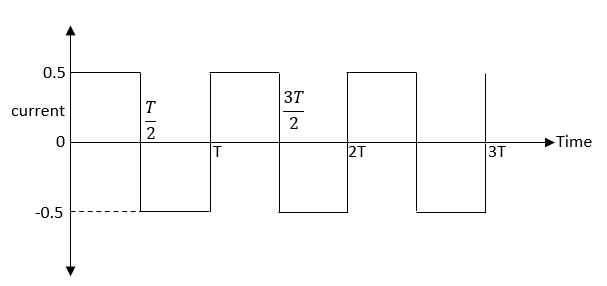
What reading would you expect of a square-wave current, switching rapidly between $ + 0.5{\text{ A}}$ and $ - 0.5{\text{ A}}$ , when passed through an AC ammeter?

Answer 1

Hint: An AC Ammeter measures the RMS value of the current passing through it. So, when a current of varying value passes through it, the AC ammeter adjusts itself such that it shows the RMS value of the current. The RMS value of AC current is defined as the current which produces the same amount of heat as a DC current of constant value when they pass through the same resistance for the same given period of time.

Complete step by step solution:
Step 1:
We know that heat produced by a current $I$ when passing through a resistor $R$ for a time $T$ is ${I^2}RT$
RMS value of Ac current is defined as the current which produces the same amount of heat as a DC current of constant value when they pass through the same resistance for the same given period of time. Let this current be ${I_{RMS}}$ .
Also assume that the current is passing through a resistor of resistance $R$
The heat produced when ${I_{RMS}}$ flows through a resistor $R$ for time $T$ is $I_{RMS}^2RT$
Step 2:
Let us assume that the current at any given point of time be $I$
Also assume that the current is passing through a resistor of resistance $R$
So, for thus given current heat produced at an instant of time $dt$ is ${I^2}Rdt$
For a continuous time period of time $T$ the heat produced will be $\int\limits_0^T {{I^2}Rdt} $
$Heat{\text{ Produced}} = \int\limits_0^T {{I^2}Rdt} $

Step 3:
As we can see that the given current varies with time.
So, to find the total heat produced, we can divide the heat produced for a cycle of $\dfrac{T}{2}$
We get the equation as,
${\text{Heat Produced}} = \int\limits_0^{\dfrac{T}{2}} {{I^2}Rdt{\text{ + }}\int\limits_{\dfrac{T}{2}}^T {{I^2}Rdt} } $
Since $I = 0.5$ from $0$ to $T$ and $I = - 0.5$ from $\dfrac{T}{2}$ to $T$
$ \Rightarrow \int\limits_0^{\dfrac{T}{2}} {{{\left( {0.5} \right)}^2}Rdt} {\text{ + }}\int\limits_{\dfrac{T}{2}}^T {{{\left( { - 0.5} \right)}^2}Rdt} $
Upon integrating the above equation, we get
$ \Rightarrow {\left( {0.5} \right)^2}R\left[ T \right]_0^{\dfrac{T}{2}}{\text{ + }}{\left( { - 0.5} \right)^2}R\left[ T \right]_{\dfrac{T}{2}}^T$
$ \Rightarrow {\left( {0.5} \right)^2}R\left[ {\dfrac{T}{2}} \right] + {\left( { - 0.5} \right)^2}R\left[ {\dfrac{T}{2}} \right]$
$ \Rightarrow 2 \times \left( {{{\left( {0.5} \right)}^2}R\dfrac{T}{2}} \right)$
$ \Rightarrow {\left( {0.5} \right)^2}RT$
Comparing this with the heat produced by a similar DC source to get ${I_{RMS}}$
$ \Rightarrow I_{RMS}^2RT = {\left( {0.5} \right)^2}RT$
$ \Rightarrow {I_{RMS}} = 0.5{\text{ A}}$

Note: Here we directly found out that the ${I_{RMS}} = 0.5$ without much effort. But in some cases where resistance and current may vary sinusoidally, linearly or in other forms. We should be careful in dividing the time into intervals which gives us easy and accurate results.